RECAP: Offline Advantage-Based Policy Optimization#

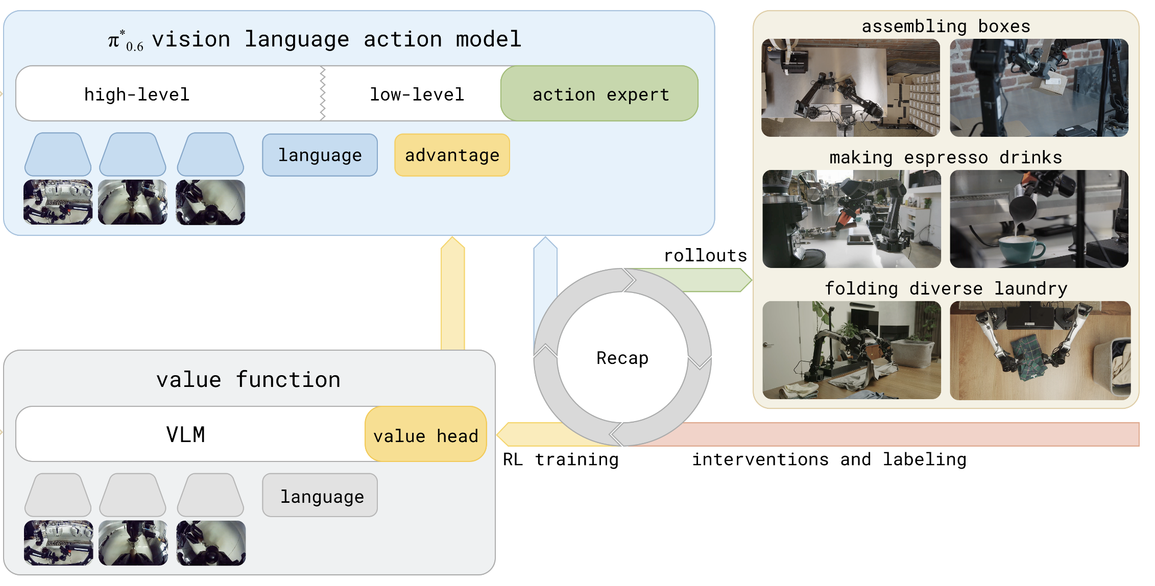
This document provides a complete guide to the RECAP (RL with Experience and Corrections via Advantage-conditioned Policies) pipeline in the RLinf framework. RECAP is an offline policy optimization method that requires no online environment interaction. It computes returns from existing datasets, trains a value model, estimates advantages, and finally uses Classifier-Free Guidance (CFG) training to optimize the policy.

This pipeline is especially suited for real-robot scenarios where large-scale online sampling is impractical.

Pipeline Overview#

RECAP consists of four sequential stages:

┌──────────────────────┐     ┌──────────────────────┐     ┌────────────────────────┐     ┌──────────────────────┐
│  Step 1              │     │  Step 2              │     │  Step 3                │     │  Step 4              │
│  Compute Returns     │────▶│  Value Model SFT     │────▶│  Compute Advantages    │────▶│  CFG Training        │
│                      │     │                      │     │                        │     │                      │
│  Compute discounted  │     │  Train a value model │     │  Compute per-timestep  │     │  Train the policy    │
│  returns for each    │     │  to predict returns  │     │  advantages using the  │     │  with classifier-    │
│  trajectory          │     │  from observations   │     │  trained value model   │     │  free guidance       │
└──────────────────────┘     └──────────────────────┘     └────────────────────────┘     └──────────────────────┘

Core Idea

Compute Returns: For each trajectory, compute discounted returns in reverse using \(G_t = r_t + \gamma \cdot G_{t+1}\), generating sidecar files without modifying the original data.
Value Model SFT: Train a value model (VLM backbone + Value Head) to predict normalized returns from observations (images + language instructions).
Compute Advantages: Use the trained value model to compute per-timestep advantages via \(A_t = \text{normalize}(r_{t:t+N}) + \gamma^N \cdot V(o_{t+N}) - V(o_t)\), then label samples as positive/negative based on a quantile threshold.
CFG Training: Train the policy model using advantage labels — positive (high-advantage) samples serve as conditional inputs and negative (low-advantage) samples as unconditional inputs, enabling classifier-free guidance for policy optimization.

Algorithm#

RECAP Core Components

Return Computation
- For SFT datasets (all successful trajectories): per-step reward \(r_t = -1\), terminal step \(r_T = 0\)
- For rollout datasets (containing failures): failed trajectory terminal step \(r_T = r_{\text{fail}}\) (e.g., \(-300\))
- Discount factor \(\gamma\) defaults to \(1.0\) (undiscounted)
Value Model
- Based on SigLIP2 vision encoder + Gemma3 language model + learnable Critic Expert
- Uses Categorical Value Distribution with 201 bins by default
- Output range \([-1, 0]\) (normalized return space)
Advantage Estimation
- N-step lookahead advantage: \(A_t = \text{normalize}(r_{t:t+N}) + \gamma^N \cdot V(o_{t+N}) - V(o_t)\)
- Quantile threshold: top \(X\%\) of samples labeled as positive (default \(X = 30\))
- Supports multi-GPU distributed inference
Classifier-Free Guidance (CFG) Training
- Based on the OpenPI (pi0.5) policy model
- positive_only_conditional mode: only positive samples serve as conditional inputs; negative samples are always unconditional
- Positive samples are randomly dropped to unconditional with probability unconditional_prob (default \(0.1\)) for dropout regularization
- At inference time, cfgrl_guidance_scale controls the guidance strength

Dependency Installation#

1. Clone RLinf Repository#

# For mainland China users, you can use the following for better download speed:
# git clone https://ghfast.top/github.com/RLinf/RLinf.git
git clone https://github.com/RLinf/RLinf.git
cd RLinf

2. Install Dependencies#

Option 1: Docker Image

docker run -it --rm --gpus all \
   --shm-size 20g \
   --network host \
   --name rlinf \
   -v .:/workspace/RLinf \
   rlinf/rlinf:agentic-rlinf0.2-maniskill_libero
   # For mainland China users, you can use the following for better download speed:
   # docker.1ms.run/rlinf/rlinf:agentic-rlinf0.2-maniskill_libero

Please switch to the OpenPI virtual environment via the built-in switch_env utility:

source switch_env openpi

Option 2: Custom Environment

# For mainland China users, you can add the `--use-mirror` flag to the install.sh command for better download speed.

bash requirements/install.sh embodied --model openpi --env maniskill_libero
source .venv/bin/activate

Model Download#

The RECAP pipeline requires the following pretrained models:

SigLIP2-so400m: Vision encoder for Step 2 value model training
Gemma3-270M: Language model for Step 2 value model training
pi0.5 base (PyTorch): Policy model for Step 4 CFG training. Refer to openpi for obtaining model weights and converting to PyTorch format

Models for Step 2

# Download models (choose either method)
# Method 1: Using git clone
git lfs install
git clone https://huggingface.co/google/siglip2-so400m-patch14-224
git clone https://huggingface.co/google/gemma-3-270m

# Method 2: Using huggingface-hub
# For mainland China users, you can use the following for better download speed:
# export HF_ENDPOINT=https://hf-mirror.com
pip install huggingface-hub
hf download google/siglip2-so400m-patch14-224 --local-dir siglip2-so400m-patch14-224
hf download google/gemma-3-270m --local-dir gemma-3-270m

After downloading, make sure to correctly specify the model paths in the configuration files:

# Step 2 value model configuration
actor:
  model:
    siglip_path: /path/to/siglip2-so400m-patch14-224
    gemma3_path: /path/to/gemma-3-270m
    tokenizer_path: /path/to/gemma-3-270m

# Step 4 policy model configuration
actor:
  model:
    model_path: /path/to/pi05_base_pytorch

Data Preparation#

RECAP uses datasets in the LeRobot format. Datasets are categorized into two types:

SFT datasets: Successful trajectories from human demonstrations or trained policies
Rollout datasets: Trajectories collected from online interaction, containing both successes and failures

Example dataset configuration:

data:
  train_data_paths:
    - dataset_path: /path/to/sft_dataset
      type: sft                # all successful trajectories
      weight: 1.0
    - dataset_path: /path/to/rollout_dataset
      type: rollout            # contains failures
      weight: 1.0

Note

train_data_paths is a list. If you want to mix multiple datasets, you can add more items; if you want to train with only one dataset, you can also keep just a single item. The train_data_paths should remain consistent across all steps to ensure returns, values, and advantages are computed on the same data.

Pipeline Tag System#

RECAP uses tags for data passing and version management across steps:

returns_tag: Generated by Step 1, read by Steps 2 and 3. Ensure that Step 1’s data.tag, Step 2’s data.tag, and Step 3’s advantage.returns_tag are consistent.
advantage_tag: Generated by Step 3, read by Step 4. Ensure that Step 3’s advantage.tag and Step 4’s data.advantage_tag are consistent.

**Tag Flow Across Pipeline Steps**#
Step	Config Field	Description
1	`data.tag`	Writes `meta/returns_{tag}.parquet`
2	`data.tag`	Reads `meta/returns_{tag}.parquet`
3	`advantage.returns_tag`	Reads `meta/returns_{tag}.parquet`
3	`advantage.tag`	Writes `meta/advantages_{tag}.parquet`
4	`data.advantage_tag`	Reads `meta/advantages_{tag}.parquet`

Step 1: Compute Returns#

This step computes discounted cumulative returns for each trajectory in reverse order. Results are saved as sidecar files without modifying the original data.

Configuration

The configuration file is located at examples/recap/process/config/compute_returns.yaml:

data:
  train_data_paths:
    - dataset_path: /path/to/sft_dataset
      type: sft
    - dataset_path: /path/to/rollout_dataset
      type: rollout

  gamma: 1.0              # discount factor
  failure_reward: -300.0   # terminal reward for failed trajectories
  tag: "fail300"           # output file tag
  num_workers: 128         # parallel processing threads

Key Parameters

Parameter	Default	Description
`data.gamma`	`1.0`	Discount factor. \(1.0\) means undiscounted (simple sum of future rewards)
`data.failure_reward`	`-300.0`	Penalty for failed trajectory terminal steps. Larger magnitude increases separation between success and failure returns
`data.tag`	`null`	Output file tag, generates `meta/returns_{tag}.parquet`
`data.num_workers`	`128`	Number of threads for parallel parquet file processing

Launch Command

bash examples/recap/process/run_compute_returns.sh compute_returns

Output Files

meta/returns_{tag}.parquet: Each row contains episode_index, frame_index, return, reward, prompt
meta/stats.json: Updated with return statistics (mean, std, min, max)

Verification

python3 -c "
import json
stats = json.load(open('/path/to/dataset/meta/stats.json'))
assert 'return' in stats
print('return stats:', stats['return'])
"

Step 2: Value Model SFT#

Using the returns computed in Step 1 as supervision signals, train a value model to predict normalized returns from observations (images + language instructions).

Model Architecture

The value model consists of three components:

Vision Encoder: SigLIP2-so400m (1152-dim) — processes RGB image inputs
Language Model: Gemma3-270M (640-dim) — processes language instructions
Critic Expert: Learnable expert head that maps multimodal representations to value predictions

The output is a Categorical Value Distribution over 201 bins spanning \([-1, 0]\).

Configuration

The configuration file is located at examples/recap/value/config/libero_sft_value.yaml. Key fields:

data:
  train_data_paths:
    - dataset_path: /path/to/sft_dataset
      type: sft
      weight: 1.0
      robot_type: "libero"
      model_type: "pi05"
  tag: "fail300"                     # must match Step 1 tag
  action_horizon: 10
  normalize_to_minus_one_zero: true  # normalize to [-1, 0]

  eval_data_paths:                   # optional, recommended
    - dataset_path: /path/to/eval_dataset
      max_samples: 10000
      robot_type: "libero"
      model_type: "pi05"

actor:
  micro_batch_size: 32
  global_batch_size: 256
  model:
    freeze_vlm: false         # whether to freeze VLM backbone
    value_dropout: 0.0        # Value Head dropout
  optim:
    lr: 5.0e-5               # VLM backbone learning rate
    value_lr: 1.0e-4          # Value Head learning rate
    weight_decay: 1.0e-10
    lr_warmup_steps: 500

runner:
  max_epochs: 30000
  save_interval: 3000         # checkpoint save interval

Key Parameters

Parameter	Default	Description
`data.tag`	`null`	Same tag as Step 1, used to read the corresponding `returns_{tag}.parquet`
`data.normalize_to_minus_one_zero`	`true`	Normalization mode. `true`: map to \([-1, 0]\); `false`: map to \([0, 1]\)
`actor.model.freeze_vlm`	`false`	Freeze the vision encoder. When `true`, also set `actor.fsdp_config.use_orig_params: True`
`actor.model.value_dropout`	`0.0`	Dropout rate before the Value Head
`actor.optim.lr`	`5.0e-5`	VLM backbone learning rate
`actor.optim.value_lr`	`1.0e-4`	Value Head learning rate

Launch Command

The training script automatically initializes the Ray cluster:

bash examples/recap/value/run_value_sft.sh libero_sft_value

Output

Model checkpoints saved at logs/value_sft/{config_name}-{timestamp}/value_sft/checkpoints/
TensorBoard logs

Key Metrics

train/actor/loss: Total value model training loss
train/actor/grad_norm: Gradient norm
eval/spearman_correlation: Spearman correlation coefficient measuring rank consistency between predictions and true returns

Note

After training, note the checkpoint path for Step 3. Checkpoints are located at:

logs/value_sft/{config_name}-{timestamp}/value_sft/checkpoints/global_step_{N}/actor/model_state_dict

Step 3: Compute Advantages#

Using the value model trained in Step 2, compute per-timestep advantage values for the dataset and label samples as positive/negative based on a quantile threshold.

Advantage Formula

\[A_t = \text{normalize}\left(\sum_{k=0}^{N-1} \gamma^k r_{t+k}\right) + \gamma^N \cdot V(o_{t+N}) - V(o_t)\]

where \(N\) is the lookahead steps (advantage_lookahead_step) and \(\gamma\) is the discount factor.

Configuration

The configuration file is located at examples/recap/process/config/compute_advantages.yaml:

advantage:
  value_checkpoint: /path/to/value_checkpoint
  positive_quantile: 0.3      # top 30% labeled as positive
  tag: "fail300_N10_ckpt18000_q30"
  returns_tag: "fail300"       # must match Step 1 tag
  batch_size: 1024

data:
  train_data_paths:
    - dataset_path: /path/to/sft_dataset
      robot_type: "libero"
      type: "sft"
      weight: 1.0
  advantage_lookahead_step: 10   # N-step lookahead
  gamma: 1.0

Key Parameters

Parameter	Default	Description
`advantage.value_checkpoint`	required	Path to the value model checkpoint from Step 2
`advantage.positive_quantile`	`0.3`	Positive sample ratio. \(0.3\) means the top 30% by advantage value are labeled as positive
`data.advantage_lookahead_step`	`10`	Lookahead steps \(N\), i.e., how many future steps of rewards to consider
`advantage.returns_tag`	`null`	Tag for reading the return file generated by Step 1
`advantage.tag`	`null`	Output advantage file tag, generates `meta/advantages_{tag}.parquet`

Launch Command

Supports multi-GPU distributed inference:

bash examples/recap/process/run_compute_advantages.sh compute_advantages

Output Files

meta/advantages_{tag}.parquet: Contains advantage (boolean), advantage_continuous (float), and other columns
Updated mixture_config.yaml: Records global threshold and normalization statistics

Verification

python3 -c "
import pandas as pd
df = pd.read_parquet('/path/to/dataset/meta/advantages_fail300_N10_ckpt18000_q30.parquet')
print(f'samples={len(df)}, columns={list(df.columns)}')
print(df[['advantage_continuous']].describe())
"

Step 4: CFG Training#

Using the advantage labels from Step 3, train the OpenPI policy model with classifier-free guidance.

Training Mechanism

Positive samples (advantage=True): Serve as conditional inputs
Negative samples (advantage=False): Always serve as unconditional inputs
When positive_only_conditional is enabled, positive samples are randomly dropped to unconditional with probability unconditional_prob for regularization
At inference time, the guidance scale cfgrl_guidance_scale amplifies the difference between conditional and unconditional predictions, steering the model toward high-advantage actions

Configuration

The configuration file is located at examples/recap/cfg/config/libero_cfg_openpi.yaml:

data:
  advantage_tag: "fail300_N10_ckpt18000_q30"   # must match Step 3 advantage.tag
  balance_dataset_weights: true
  train_data_paths:
    - dataset_path: /path/to/sft_dataset
      type: sft
      weight: 1.0
    - dataset_path: /path/to/rollout_dataset
      type: rollout
      weight: 1.0

actor:
  micro_batch_size: 32
  global_batch_size: 512
  model:
    model_path: /path/to/pi05_base_pytorch
    openpi:
      config_name: "pi05_libero"
      positive_only_conditional: true
      unconditional_prob: 0.1
      cfgrl_guidance_scale: 1.0
  optim:
    lr: 1.0e-5
    lr_scheduler: cosine
    lr_warmup_steps: 5000
    total_training_steps: 30000

Key Parameters

Parameter	Default	Description
`data.advantage_tag`	`null`	Matches Step 3’s `advantage.tag` for reading advantage labels
`actor.model.openpi.positive_only_conditional`	`true`	Only positive samples serve as conditional inputs. When `false`, both positive and negative samples are conditional
`actor.model.openpi.unconditional_prob`	`0.1`	Probability of dropping samples to unconditional. When `positive_only_conditional` is enabled, applies only to positive samples; otherwise applies to all samples
`actor.model.openpi.cfgrl_guidance_scale`	`1.0`	Guidance scale at inference. Higher values favor high-advantage actions more strongly
`actor.model.openpi.config_name`	`pi05_libero`	Data transform config. Use `pi05_libero` for LIBERO, `pi05_maniskill_sim_real_co_training` for Franka
`data.balance_dataset_weights`	`true`	Balance sampling weights by dataset size

Launch Command

bash examples/recap/cfg/run_cfg_sft.sh libero_cfg_openpi

Key Metrics

train/actor/loss: Policy training loss
train/actor/grad_norm: Gradient norm

Visualize Advantages#

After Step 3, use examples/recap/process/visualize_advantage_dataset.py to analyze the advantage distribution, including advantage histograms, value prediction distributions, per-episode positive rates, and episode replay videos with advantage annotations.

Basic Usage

Generate distribution plots and episode videos:

python examples/recap/process/visualize_advantage_dataset.py \
    --dataset /path/to/your/dataset \
    --output outputs/advantage_viz \
    --tag "fail300_N10_ckpt18000_q30" \
    --num-episodes 10

Distribution plot only (no videos):

python examples/recap/process/visualize_advantage_dataset.py \
    --dataset /path/to/your/dataset \
    --output outputs/advantage_viz \
    --tag "fail300_N10_ckpt18000_q30" \
    --no-video

Visualize specific episodes:

python examples/recap/process/visualize_advantage_dataset.py \
    --dataset /path/to/your/dataset \
    --output outputs/advantage_viz \
    --tag "fail300_N10_ckpt18000_q30" \
    --episodes 0 5 10 20

Key Parameters

Parameter	Default	Description
`--dataset`	required	Path to LeRobot dataset
`--output`	`outputs/advantage_viz`	Output directory
`--tag`	`null`	Advantage file tag, reads `meta/advantages_{tag}.parquet`
`--num-episodes`	`10`	Number of episodes to visualize (`0` for all)
`--episodes`	`null`	Specific episode indices to visualize
`--no-video`	`false`	Skip video generation, output static plots only
`--threshold`	auto-detected	Advantage threshold. When not set, automatically inferred from `mixture_config.yaml` or data

Output Contents

advantage_distribution.png: 6-subplot comprehensive statistics panel (advantage histogram, value distribution, scatter plot, per-episode positive rate, per-episode advantage mean, statistics summary)
episode_{N}_summary.png: Key frames + value/advantage time series for each episode (frames above threshold highlighted with green border)
episode_{N}.mp4: Per-frame replay video with advantage annotations

Visualization and Results#

TensorBoard Logging

tensorboard --logdir ./logs --port 6006

The RECAP pipeline generates two subdirectories under logs/:

logs/value_sft/: Value model training logs (Step 2)
logs/cfg_sft/: CFG policy training logs (Step 4)

Train Log Tool Integration

runner:
  logger:
    log_path: "../results"
    project_name: rlinf
    experiment_name: "recap_experiment"
    logger_backends: ["tensorboard"]   # also supports wandb, swanlab

Dataset#

We provide a reproduced experiment on the LIBERO-10 benchmark (Task 0) to demonstrate the RECAP pipeline.

SFT data: Expert demonstration data from LIBERO-10 (successful trajectories)
Rollout data: 4,096 trajectories collected by a few-shot π_0.5 policy on Task 0, containing both successful and failed episodes
Eval data: A held-out set collected by the same few-shot π_0.5 policy, used in Step 2 to monitor value model overfitting

Note

This tutorial intentionally uses a few-shot π_0.5 policy with a moderate initial success rate so that RECAP’s offline improvement can be observed in a compact Task 0 example. The baseline below is scoped to this reproduced setup; it is not intended to represent the general π_0.5 SFT performance on the full LIBERO benchmark.

The dataset is available here.

RECAP Results#

After one iteration of the RECAP pipeline on LIBERO-10 Task 0, the success rate improves from 48.8% (the few-shot SFT baseline in this tutorial setup) to 66.5% (RECAP), an absolute improvement of 17.7%.

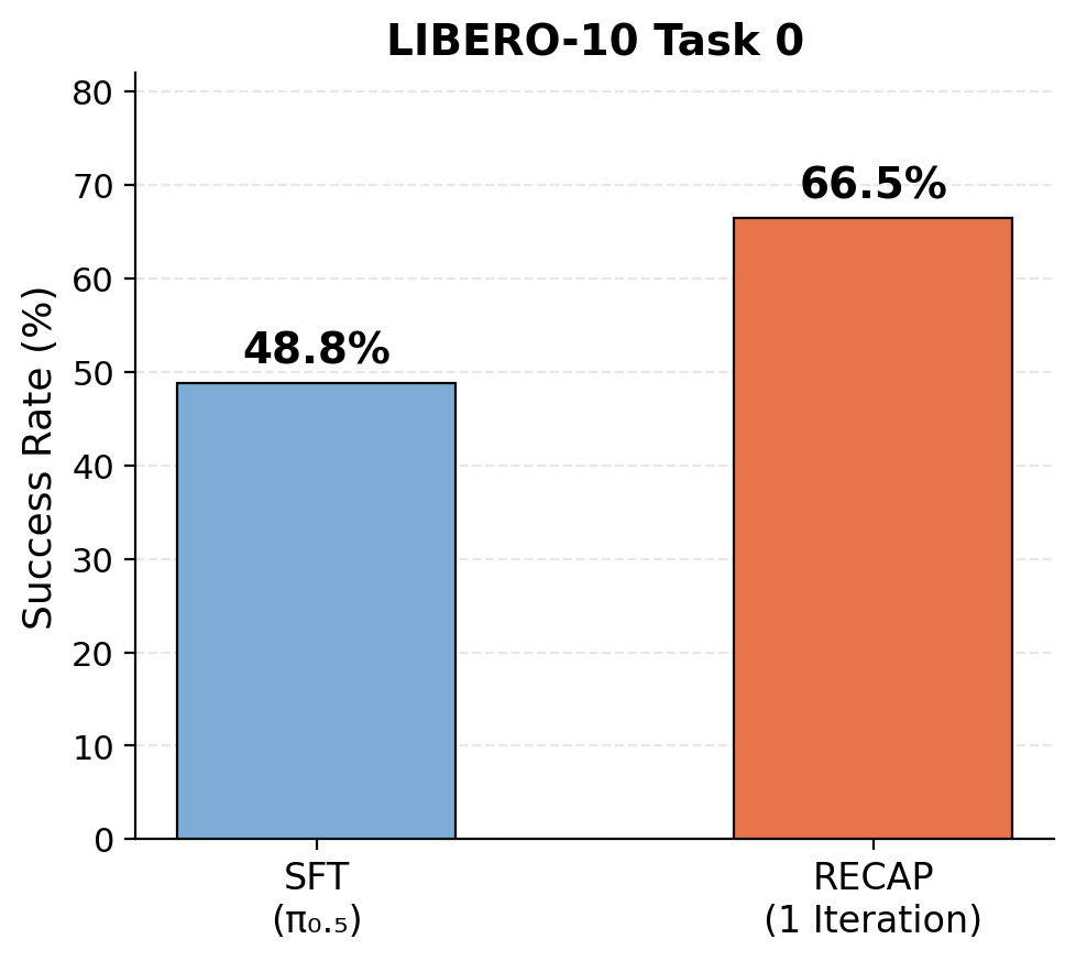
RECAP results on LIBERO-10 Task 0

Advanced Usage#

Threshold Relabeling#

To adjust the quantile threshold (e.g., from 30% to 20%) without rerunning the full Step 3, use recompute_advantages_from_value_reward.py for threshold-only relabeling:

cd examples/recap/process
python recompute_advantages_from_value_reward.py \
    --dataset_paths /path/to/sft_dataset /path/to/rollout_dataset \
    --source_tag "fail300_N10_ckpt18000_q30" \
    --new_tag "fail300_N10_ckpt18000_q20" \
    --positive_quantile 0.2

You can also use --dataset_root to specify a root directory containing multiple datasets, with --advantage_lookahead_step to recompute advantages:

python recompute_advantages_from_value_reward.py \
    --dataset_root /path/to/dataset_root \
    --advantage_lookahead_step 20 \
    --positive_quantile 0.3

This script reads existing continuous advantage values (advantage_continuous), updates only the threshold and boolean labels, avoiding redundant GPU inference.

Iterative Optimization#

RECAP supports iterative optimization: use the policy trained in Step 4 to collect new data, then restart from Step 1. Use different tags for each iteration to track results:

Iter 1: tag="fail300"          → Train Value Model → tag="fail300_N10_ckpt18000_q30"     → CFG Training
Iter 2: tag="fail300_iter2"    → Train Value Model → tag="fail300_iter2_N10_ckpt6000_q20" → CFG Training

File Structure#

examples/
└── recap/
    ├── process/
    │   ├── compute_returns.py               # Step 1: compute returns
    │   ├── compute_advantages.py            # Step 3: compute advantages
    │   ├── recompute_advantages_from_value_reward.py  # threshold relabeling
    │   ├── visualize_advantage_dataset.py    # advantage visualization
    │   ├── run_compute_returns.sh            # Step 1 launch script
    │   ├── run_compute_advantages.sh         # Step 3 launch script
    │   └── config/
    │       ├── compute_returns.yaml
    │       └── compute_advantages.yaml
    ├── value/
    │   ├── train_value.py                # Step 2: value model training
    │   ├── run_value_sft.sh              # Step 2 launch script
    │   └── config/
    │       ├── libero_sft_value.yaml
    │       └── model/
    │           └── value.yaml            # value model config
    └── cfg/
        ├── train_cfg.py                  # Step 4: CFG policy training
        ├── run_cfg_sft.sh                # Step 4 launch script
        └── config/
            └── libero_cfg_openpi.yaml